CB Radio Microphone wiring Guide

Thanks Simone IW5EDI
http://www.iw5edi.com/technical-articles/microphone-connections


Welcome, this page describes microphone wiring connections for most UK and foreign radios. Most U.S. radios are “Code Type 2″, so if the radio you want to wire a mic up for is not mentioned here, be sure to try out “Code Type 2″.
To Use this Chart: Look up your radio. To the left is a “Type” number. Look further down the Chart to CODE section. Find your number. This is your radio’s mic wiring. Further down the Chart are a few microphone’s and their wiring pinouts.  Remember that the Shield wire is most alway’s wrapped around the Audio wire.

--------------------------------------------------------------------------------

Radio                     TYPE

-------------------------------

Academy CB501             4
Academy CB502             4
Alan (Midland) 555        2
Alan {Midland) 560        15
Alba CBM1                 1
Alpha 4000                1
Amstrad CB900             4
Amstrad CB901             1
Antron CB5097             9
Atron 507                 2
Audioline 340             2
Audioline 341             2
Audioline 345             2
--------------------------------------------------------------------------------

Barracuda GT868           4
Barracuda HB940           1
Beta 1100 (Kernow)        1
Beta 2100 (Kernow)        12
Beta 3100 (Kernow)        12
Binatone 5 Star           1
Binatone Route 66         1
Binatone Speedway         1
Boman CB 515 - 525
535 - 710 - 910 - 920
930 - 950 - 970 - 990     1
Braemar PT40              1
--------------------------------------------------------------------------------

CB master 2040            17
Cheiza CB702              4
Cobra 18LTD               2
Cobra 18 PLUS             3
Cobra 18RV                3
Cobra 18ULTRA             2
Cobra 19                  2
Cobra 19DX-LTD            2
Cobra 19GTL               2
Cobra 19LTD               2
Cobra 19Plus              3
Cobra 19ULTRA             2
Cobra 19X                 3
Cobra 20 LTD              3
Cobra 20PLUS              3
Cobra 21                  2
Cobra 21GTL               2
Cobra 21LTD               2
Cobra 21LTD-CLASSIC       2
Cobra 21XFM               3
Cobra 21XLR               2
Cobra 23 PLUS             3
Cobra 25                  2
Cobra 25GTL               2
Cobra 25LTD               2
Cobra 25LTD-CLASSIC GOLD  2
Cobra 25LTD-WX CLASSIC    2
Cobra 25PLUS              2
Cobra 26                  2
Cobra 29                  2
Cobra 29LTD               2
Cobra 29LTD-CLASSIC       2
Cobra 29LTD-CLASSIC-GOLD  2
Cobra 29LTDWX CLASSIC     2
Cobra 29PLUS              2
Cobra 29XLR               2
Cobra 31PLUS              2
Cobra 33PLUS              2
Cobra 40X                 2
Cobra 41 PLUS             3
Cobra 77X                 2
Cobra 78X                 2
Cobra 86XLR               2
Cobra 87GTL               2
Cobra CAM-89              2
Cobra 89GTL               2
Cobra 89XLR               2
Cobra 90                  14
Cobra 90 LTD              14
Cobra 93LTD-WX            2
Cobra 135                 2
Cobra 135XLR              2
Cobra 138XLR              2
Cobra 139XLR              2
Cobra 140GTL              14
Cobra 142GTL              14
Cobra 148GTL              14
Cobra 146GTL              2
Cobra 148-F-GTL           14
Cobra 148GTL-B            2
Cobra 148GTL-DX           2
Cobra 1000GTL             2
Cobra 2000GTL             14
Cobra 2010                14
Colt 210                  17
Colt 220                  17
Colt 222                  17
Colt 290                  1
Colt 295                  3
Colt 390 - 480 - 485      1
Colt 510                  17
Colt 800 - 870
1000 - 1200 - 2400        1
Commtel GT858             4
Commtel GT868             4
Commtron CB40F            3
Commtron CXX              17
Commtron X11              17
Communicator NI440DX      1
Compact 40                1
Connex 3300               2
Consam 1320               1
Courier Galaxy            14
Craig L193                2
Craig L101 - L102         19
Craig L104                2
Craig L131                18
Craig L232                14
Craig L231 - L331         14
Craig 4101 - 4102
4103 - 4104 - 4201        19
Cybernet Beta 1000        1
Cybernet Beta 2000        1
Cybernet Beta 3000        1
Cybernet Delta 1          1
--------------------------------------------------------------------------------

Danita 440                7
Danita 640                2
Dirland 77-099            2
Dirland SuperStar 3900    2
Dirland SuperStar 3900B   2
DNT M40                   5
DNT B40FM                 5
Domico Convoy 1           1
--------------------------------------------------------------------------------

Eagle 2000                2
Eagle 5000                15
Elftone                   4
Emperor TS-5010           16
Eurosonic ES404           1
Eurosonic Euro II         1
Eurosonic GT868           1
--------------------------------------------------------------------------------

Falcon FCB1281            1
Fidelity CB1000FM         4
Fidelity CB2000FM         1
Fidelity CB2001FM         1
Fidelity 3000FM           4
Ford Roadmaster 505       1
Formac 88-120             1
Formac 88 (5 pin)         17
--------------------------------------------------------------------------------

Galaxy DX33HML            2
Galaxy 33Plus             2
Galaxy DX44V              2
Galaxy DX55               2
Galaxy DX66V              2
Galaxy DX77HML            2
Galaxy DX77V              2
Galaxy DX88HML            2
Galaxy 2100               2
Galaxy Jupitor            2
Galaxy Mars               2
Galaxy Mirage             2
Galaxy Mirage 44          2
Galaxy Pluto              2
Galaxy Saturn             2
Galaxy Saturn 2           2
Galaxy Sirius             2
Galaxy Super Galaxy       2
Gecol                     4
Grandstand Base           9
Grandstand Bluebird       7
Grandstand Gemini         7
Grandstand Hawk           1
--------------------------------------------------------------------------------

Ham International (all)   1
Harrier CB                1
Harier CBX                1
Harier HQ                 1
Harry Moss 325            2
Havard 402 (H160)         1
Havard H403 G/Buddy       11
Havard H404               1
Havard H407               1
Havard 420M (H405)        1
Havard H646               1

 

--------------------------------------------------------------------------------

Icom ICB1050              1
Interceptor TC300         1
--------------------------------------------------------------------------------

Jesan KT200               1
Jesan KT4004              1
Jesan KT 7007             1
Jesan Pro 8000            1
Johnstone                 4
JWR M2                    1
--------------------------------------------------------------------------------

Kestral                   1
Kraco 4004                2
Kraco 4030                1

--------------------------------------------------------------------------------

Lake Manxman 850          4
Lake Manxman 950          4
Lancaster                 1
LCL 2740                  5
LCL Economy               5
LCL Enterprise            5
Legionairre               11
Lowe TX40                 3
--------------------------------------------------------------------------------

Manor Kestrel             1
Maxcom 6E                 3
Maxcom Appolo 16E         3
Maxcom 20E                3
Maxcom 21E                3
Maxcom 30E                1
Maxon MX1000              12
Maxon MX2000              12
Maycom EM27               12
Midland 2001              1
Midland 3001              1
Midland 4001              1
Midland 77-095            1
Midland 77-099            3
Midland 77-104            3
Midland 77-805            13
Midland Power Max         1
Moonraker Major           1
Moonraker Minor           1
Murphy CBH1500            20
Murphy CBH1500            10
Murphy DS602              1
Mustang CB1000            1
Mustang CB2000            1
Mustang CB3000            1
--------------------------------------------------------------------------------

Nato 2000                 1
Nentone                   3
--------------------------------------------------------------------------------

Pama GX19                 1
Pama GX25                 1
Pama GX1000               1
Pama GX2000               1
Planet 2000               1
Pyramid 1300              2
Pyramid CB-22             1
Pyramid CB-24             1
Pyramid CB-25             1
Pyramid CB-26             1
Pyramid CB-28             1
--------------------------------------------------------------------------------

Radiomobile CB201         1
Radiotechnic RT852        5
Ranger 2950               15
Ranger 2970               15
Ranger 2900               15
Ranger 2990               15
Realistic TRC2000         6
Realistic TRC2001         6
Realistic TRC2002         6
Realistic TRC3000         6
Reftec 934                1
Rotel RVC220              1
Rotel RVC230              1
Rotel RVC240              1
--------------------------------------------------------------------------------

Sapphire X2000            4
Sapphire X4000            1
Satcom Scan 40F           1
Satcom Scan 4000          1
Shogun                    8
Sirtel Searcher           3
SMC Oscar 1               1
SMC Oscar 2               1
Spinneytronic CB199       1
Sun 401                   1
Superstar 2000            1
--------------------------------------------------------------------------------

Team Eurocontrol          12
Team Euro 3004            12
Team Euro 3100UK          1
Team TRX404               1
Team TRX404UK             1
Team TS290                12
Team TS1000               3
Team TSM404               1
Telecom TC900             21
Transcom GBX4000          1
Transcom 1000,2000,3000   1
--------------------------------------------------------------------------------

Uniden 100                2
Uniden 200                2
Uniden 300                2
Uniace 400 (934)          1
Uniden 400 (cept)         2
Uniden PC404              2
Uniden PRO 420E           2
Uniden PRO 450E           2
Uniden PRO 620E           2
Uniden HR-2510            16
Uniden HR-2600            16
Uniden Grant XL           14
Uniden Lincoln            16
Uniden Washington         14
--------------------------------------------------------------------------------

Viper 88                  1
--------------------------------------------------------------------------------

Wagner 506                9
--------------------------------------------------------------------------------

York JCB861               1
York JCB863               1
York JCB867               1
--------------------------------------------------------------------------------

Zodiac M144               7
Zodiac M244               7

--------------------------------------------------------------------------------
Wiring Codes Explained:
Type 1
1 = Audio
2 = Ground / Common
3 = Receive
4 = Transmit

Type 2
1 = Ground / Common
2 = Audio
3 = Transmit
4 = Receive

Type 3
1 = Audio
2 = Transmit
3 = N/C
4 = Ground / common
5 = Receive

Type 4
1 = Receive
2 = Transmit
3 = Audio
4 = Ground / Common

Type 5
1 = Audio
2 = N/C
3 = Transmit
4 = Ground / Common
5 = N/C

Type 6
1 = Ground / common
2 = N/C
3 = Transmit
4 = Audio
5 = Receive

Type 7
1 = Audio
2 = Ground / Common
3 = Transmit
4 = N/C
5 = Receive

Type 8
1 = Audio
2 = Ground / Common
3 = Transmit
4 = Receive
5 = 12 Volt Feed

Type 9
1 = Ground / Common
2 = Audio
3 = Transmit
4 = N/C

Type 10
1 = Recieve
2 = Ground / Common (Linked)
3 = Transmit
4 = Audio

Type 11
1 = Audio
2 = Ground / Common
3 = Transmit
4 = Receive

Type 12
1 = Audio
2 = Receive
3 = Transmit
4 = Down/Up
5 = Ground / Common
6 = N/C or volts

Type 13
1 = Transmit
2 = Receive
3 = N/C
4 = Ground / Common
5 = Audio

Type 14
1 = Audio
2 = Ground / Common
3 = Receive
4 = Switching Wire
5 = Transmit

Type 15
1 = Ground / Common
2 = Audio
3 = Transmit
4 = Receive
5 = Channel Up
6 = Channel Down

Type 16
1 = Audio
2 = Ground / Common
3 = Transmit
4 = Channel Up
5 = Channel Down

Type 17
1 = Audio
2 = Transmit
3 = Shield
4 = N/C
5 = Receive

Type 18
1 = N/C
2 = Audio
3 = Receive
4 = Shield
5 = Transmit

Type 19
1 = N/C
2 = Audio
3 = Shield
4 = Receive
5 = Transmit

Type 20
1,2 = Screen
3 = Transmit
4 = Audio
Type 21
1 = Audio
2 = Screen
3 = Transmit
4 = Receive
5 = n/c
 

Microphone Colour Codes

Altai(All)

Shield = Ground
Black = Common
Red = Mic or Audio
White = TX
Blue = RX

 

Astatic 4 Wire
575M, D104M, TUG-8,

Shield= Common
White= Mic or Audio
Red= Tx
Black= Rx

 

Astatic 6 Wire
575M-6, 636L,D104M-6, M6B,1104C/CM,
T-UG9, T-UP9, Diamond/Golden Eagle,
Night K/Silver K Eagle, Road Devil

Shield = Ground
Blue = Common
White = Mic or Audio
Red = TX
Black = RX
Yellow = Audio Switch

 

Cobra
CA- 70 /71 / 72 / 79 / 80

Shield = Ground
Black = Common
Red = Mic or Audio
White = Tx.
Blue = Rx.
CTE F10 & F16

Shield = Common
Blue = Mic or Audio
White = TX
Red = RX

 

Daiwa
EM-500

Shield = Ground
Black = Common
Red = Mic or Audio
White = Tx.
Blue = Rx.

 

Galaxy
DC-521S (4 Wire)

Shield = Common
Yellow = Mic or Audio
Red = Tx.
Black = Rx.

 

Galaxy
CB-660EI / EIR

Shield = Ground
Black = Common
White = Mic or Audio
Red = Tx.
Blue = Rx

 

Heatherlite

Shield = Common
White = Mic or Audio
Red = TX
Black = RX

 

K40

Shield = Ground
Black = Common
White = Mic or Audio
Red = TX
Blue = RX
Yellow = Audio Switch

 

Realistic 5 wire

Shield = Common
White = Mic or Audio
Red = TX
Black = RX
Blue = Audio Switch

 

Sadelta (All)
Bravo Plus, EchoMaster +/ Pro,
ME-3, MB-4, MB-4 W/R.B.

Shield = Common
White = Mic or Audio
Brown = TX
Green = RX

 

Turner 3 Wire

Shield = Common
White = Mic or Audio
Black = TX
Red = RX

 

Turner 6 Wire
Expander 500, Road Kink 56 / 76

Shield = Shield
Red = Common
White = Mic Or Audio
Blue = TX
Black = RX
Yellow = Audio Switch

 

Valor

PDC-66/67
Shield= Common
White= Mic or Audio
Red= Tx
Black= Rx

Zetagi

Shield = Common
Yellow = Audio
Black = TX
Red = RX

26CT1316 Keith's Homebrew Antennas

Maltese 2 element Yagi 

Maltese 2 element Yagi 

Maltese 2 element Quad 

Spiral Beam and Maltese 2 element Quad

Plans for 2 element beam 

Plans for 2 element cubical quad

Mark 26MA090 Home Brew SS360 in Marantz Chassis

Climbing up the Russian Woodpecker DUGA 3 Chernobyl-2 OTH radar Залаз на ЗГРЛС Чернобыль-2 "ДУГА"

Published on Dec 7, 2013

20 min HD of climbing up the Russian Woodpecker (over-the-horizon radar station).
Join us at http://forum.pripyat.de/
Report from Chernobyl-2 OTH radar station: http://pripyat.de/chernobyl2.htm (only in german)

From Wikipedia, the free encyclopedia

 Duga-3 Russian: Дуга-3 (NATO reporting name Steel Yard) was a Soviet over-the-horizon (OTH) radar system used as part of the Soviet ABM early-warning network. The system operated from July 1976 to December 1989. Two Duga-3 radars were deployed, one near Chernobyl and Chernihiv, the other in eastern Siberia.

The Duga-3 systems were extremely powerful, over 10 MW in some cases, and broadcast in the shortwave radio bands. They appeared without warning, sounding like a sharp, repetitive tapping noise at 10 Hz,^[1] which led to it being nicknamed by shortwave listeners the Russian Woodpecker. The random frequency hops disrupted legitimate broadcast, amateur radio, commercial aviation communications, utility transmissions, and resulted in thousands of complaints by many countries worldwide. The signal became such a nuisance that some receivers such as amateur radios and televisions actually began including 'Woodpecker Blankers' in their design.
The unclaimed signal was a source for much speculation, giving rise to theories such as Soviet mind control and weather control experiments. However, many experts and amateur radio hobbyists quickly realized it to be an OTH system. NATO military intelligence had already photographed the system and given it the NATO reporting name Steel Yard. This theory was publicly confirmed after the fall of the Soviet Union.

Contents

• 1 History
  • 1.1 Genesis
  • 1.2 Russian Woodpecker
  • 1.3 Civilian identification
  • 1.4 Jamming
  • 1.5 Disappearance
• 2 Locations
• 3 Appearances in media
• 4 See also
• 5 References
• 6 Further reading
• 7 External links

History

Genesis

The Soviets had been working on early warning radar for their anti-ballistic missile systems through the 1960s, but most of these had been line-of-sight systems that were useful for raid analysis and interception only. None of these systems had the capability to provide early warning of a launch, within seconds or minutes of a launch, which would give the defences time to study the attack and plan a response. At the time the Soviet early-warning satellite network was not well developed, and there were questions about their ability to operate in a hostile environment including anti-satellite efforts. An over-the-horizon radar sited in the USSR would not have any of these problems, and work on such a system for this associated role started in the late 1960s.
The first experimental system, Duga-1, was built outside Mykolaiv in Ukraine, successfully detecting rocket launches from Baikonur Cosmodrome at 2,500 kilometers. This was followed by the prototype Duga-2, built on the same site, which was able to track launches from the far east and submarines in the Pacific Ocean as the missiles flew towards Novaya Zemlya. Both of these radar systems were aimed east and were fairly low power, but with the concept proven work began on an operational system. The new Duga-3 systems used a transmitter and receiver separated by about 60 km.^[2]

	Woodpecker Menu 0:00 Woodpecker on shortwave radio interfering with WWVH, November 2, 1984.
Problems playing this file? See media help.

Duga-3 array within the Chernobyl Exclusion Zone. The array of pairs of cylindrical/conical cages on the right are the driven elements, fed at the facing points with a form of ladder line

Transmitter

Receiver

Russian Woodpecker in Kiev Oblast

Russian Woodpecker

Starting in 1976 a new and powerful radio signal was detected worldwide, and quickly dubbed the Woodpecker by amateur radio operators. Transmission power on some woodpecker transmitters was estimated to be as high as 10 MW equivalent isotropically radiated power.^{[citation needed]}
Triangulation quickly revealed the signals came from Ukraine. Confusion due to small differences in the reports being made from various military sources led to the site being alternately located near Kiev, Minsk, Chernobyl, Gomel or Chernihiv. All of these reports were describing the same deployment, with the transmitter only a few kilometers southwest of Chernobyl (south of Minsk, northwest of Kiev) and the receiver about 50 km northeast of Chernobyl (just west of Chernihiv, south of Gomel). Unknown to civilian observers at the time, NATO was aware of the new installation^{[citation needed]}, which they referred to as Steel Yard.

Civilian identification

Even from the earliest reports it was suspected that the signals were tests of an over-the-horizon radar,^[3] and this remained the most popular hypothesis during the Cold War. Several other theories were floated as well, including everything from jamming western broadcasts to submarine communications. The broadcast jamming theory was debunked early on when a monitoring survey showed that Radio Moscow and other pro-Soviet stations were just as badly affected by woodpecker interference as Western stations.
As more information about the signal became available, its purpose as a radar signal became increasingly obvious. In particular, its signal contained a clearly recognizable structure in each pulse, which was eventually identified as a 31-bit pseudo-random binary sequence, with a bit-width of 100 μs resulting in a 3.1 ms pulse.^[4] This sequence is usable for a 100 μs chirped pulse amplification system, giving a resolution of 15 km (10 mi) (the distance light travels in 50 μs). When a second Woodpecker appeared, this one located in eastern Russia but also pointed toward the US and covering blank spots in the first system's pattern, this conclusion became inescapable.
In 1988, the Federal Communications Commission conducted a study on the Woodpecker signal. Data analysis showed an inter-pulse period of about 90 ms, a frequency range of 7 to 19 MHz, a bandwidth of 0.02 to 0.8 MHz, and typical transmission time of 7 minutes.

• The signal was observed using three repetition rates: 10 Hz, 16 Hz and 20 Hz.
• The most common rate was 10 Hz, while the 16 Hz and 20 Hz modes were rather rare.
• The pulses transmitted by the woodpecker had a wide bandwidth, typically 40 kHz.

Jamming

The array at Chernobyl, viewed from a distance

To combat this interference, amateur radio operators attempted to "jam" the signal by transmitting synchronized unmodulated continuous wave signals at the same pulse rate as the offending signal. They formed a club called The Russian Woodpecker Hunting Club.^[5]

Disappearance

Starting in the late 1980s, even as the U.S. Federal Communications Commission (FCC) was publishing studies of the signal, the signals became less frequent, and in 1989, they disappeared altogether. Although the reasons for the eventual shutdown of the Duga-3 systems have not been made public, the changing strategic balance with the end of the Cold War in the late 1980s likely had a major part to play. Another factor was the success of the US-KS early-warning satellites, which entered preliminary service in the early 1980s, and by this time had grown into a complete network. The satellite system provides immediate, direct and highly secure warnings, whereas any radar-based system is subject to jamming, and the effectiveness of OTH systems is also subject to atmospheric conditions.
According to some reports, the Komsomolsk-na-Amure installation in the Russian Far East was taken off combat alert duty in November 1989, and some of its equipment was subsequently scrapped. The original Duga-3 site lies within the 30 kilometer Zone of Alienation around the Chernobyl power plant. It appears to have been permanently deactivated, since their continued maintenance did not figure in the negotiations between Russia and Ukraine over the active Dnepr early warning radar systems at Mukachevo and Sevastopol. The antenna still stands, however, and has been used by amateurs as a transmission tower (using their own antennas) and has been extensively photographed.

Locations

Soviet over-the-horizon radar stations Duga-1 and Duga-2 Mykolaiv transmitter at 46°48′26″N 32°13′12″E receiver at 47°02′28.33″N 32°11′57.29″E Duga-3 (western) Liubech and Chernobyl-2 transmitter at 51°18′19.06″N 30°03′57.35″E receiver at 51°38′15.98″N 30°42′10.41″E Duga-3 (eastern) Komsomolsk-na-Amure transmitter at 50°23′07.98″N 137°19′41.87″E receiver at 50°53′34.66″N 136°50′12.38″E Radar Over-the-horizon radar Missile defense

Appearances in media

The Ukrainian-developed computer game S.T.A.L.K.E.R. has a plot focused on the Chernobyl Nuclear Power Plant and the nuclear accident there. The game heavily features actual locations in the area, including the Duga-3 array. The array itself appears in STALKER: Clear Sky in the city of Limansk-13. While the 'Brain Scorcher' from STALKER: Shadow of Chernobyl was inspired by theories that Duga-3 was used for mind control, it does not take the form of the real array.
In Call of Duty: Black Ops, the Grid map is placed in Pripyat near the DUGA-3 array.
In the movie Divergent, the wall around Chicago is derived from photographs of the Duga-3 array.^[6]

See also

• Cobra Mist
• Jindalee Operational Radar Network
• Numbers station
• UVB-76

References

1. 
   

David L. Wilson (Summer 1985). "The Russian Woodpecker... A Closer Look". Monitoring Times. Retrieved 2007-06-15.

Bukharin, Oleg; et al. (2001). Pavel Podvig, ed. Russian Strategic Nuclear Forces. Cambridge, Massachusetts: MIT Press.

"Mystery Soviet over-the-horizon tests". Wireless World: 53. February 1977. Retrieved 2007-06-15.

J.P. Martinez (April 1982). "Letter from J. P. Martinez". Wireless World: 89. Retrieved 2007-06-15.

Dave Finley (7 July 1982). "Radio hams do battle with 'Russian Woodpecker'". The Miami Herald. Retrieved 2007-06-15.

6. The "Woodpecker" moves to fururistic Chicago! //QRZ.com; The Russian Woodpecker = the wall around Chicago in Divergent; Marcel Birgelen : "thing is surrounded by a great wall, which has some eery similarities to the Russian Woodpecker."

Further reading

• Headrick, James M. (1 July 1990). "Looking over the horizon (HF radar)". IEEE Spectrum 27 (7): 36–39. doi:10.1109/6.58421.
• Headrick, James M.; Skolnik, Merrill I. (1 January 1974). "Over-the-Horizon radar in the HF band". Proceedings of the IEEE 62 (6): 664–673. doi:10.1109/PROC.1974.9506.
• Headrick, James M., Ch. 24: "HF over-the-horizon radar," in: Radar Handbook, 2nd ed., Merrill I. Skolnik, ed. [New York: McGraw-Hill, 1990].
• Kosolov, A. A., ed. Fundamentals of Over-the-Horizon Radar (translated by W. F. Barton) [ Norton, Mass.: Artech House, 1987].
• John Pike. "Steel Yard OTH". GlobalSecurity.org. Retrieved 2010-04-08.

Chirp Sounding

Passive Ionospheric Sounding and Ranging

From QSL.net

Chirp Sounding is a relatively new technique used to measure the ionosphere by bouncing signals off it, in much the same way as a RADAR system. Indeed, older Ionosondes (equipment for sounding the ionosphere) worked in exactly that way, by sending high powered pulses and listening for the response. The modern Chirp Sounder uses lower power and a continuous signal which changes frequency at a steady rate. Background
Peter Martinez G3PLX and others have used Digital Signal Processing (DSP) and Doppler techniques to measure small differences in carrier frequency that result from movements in the radio propagation path (see the Precision Carrier Analysis page). While interesting for meteor scatter, aircraft and satellite reflections, and more gross or localized ionospheric effects, this technique gives no direct information about reflection layer height, and it becomes difficult to infer information about the propagation medium over more complex paths. What was required was a time domain - rather than frequency domain - technique, for example measuring the propagation time of pulses. It was soon established that a wideband technique, rather than a carrier based technique would be necessary, in order to achieve sufficient time resolution.
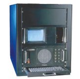
In searching for suitable pulse transmissions to use, preferably transmissions available from all over the world on a 24 hour basis, Peter stumbled across a family of transmitters that are used as swept frequency ionospheric sounders. In their normal application, research, professional and military groups use these low power devices to probe the ionosphere to measure propagation. The signal consists of a single long 'chirp', sweeping up in frequency at a constant rate, and repeated periodically. These transmissions are tracked by a companion receiver which is zero beat with the transmitter, and so ionospheric reflections that are returned with short delays are heard as lower sideband audio beats of a few hundred Hz. The equipment then builds an 'ionogram' or two dimensional graphical representation of the ionosphere's reflection height or delay against frequency. The adjacent picture illustrates a typical commercial 50W FM/CW (chirped) ionospheric sounding transmitter.
The first step was to discover how these chirped signals could be used in a passive manner, i.e. without reference to the transmitter oscillators or timing reference. To do this, Peter developed a very clever chirped filter, which not only sweeps in frequency at 100 kHz/second, but has properties not possible in a conventional filter - a bandwidth of only 66 Hz, but with a pulse resolution of 0.66ms. This filter and matching detection software formed the basis of the adventure to follow, and allowed these chirped sounders to be analysed on a single frequency using a fixed receiver. The remaining problem was to determine when the chirp transmissions started, in order to know when it should sweep past the receiver, in order to calibrate the fixed frequency receiver for range.
Purpose
The purpose of this project has been to explore the use of publicly available chirped ionospheric sounding transmissions to study the ionosphere. We now know that these transmissions are made regularly from most parts of the world, and cover much of the HF spectrum from about 3 to 30 MHz on a 24 hour basis. The unique aspect of this project is that it is wholly passive - it makes use of the sounding transmissions made by other agencies. This means that anyone can potentially receive and interpret the transmissions.
The transmissions used by this project are chirped sounders which transmit at a constant rate of 100 kHz/second, and have reliable chirp start times. Most of these sounders are commercial and research transmissions for vertical or oblique ionospheric sounding purposes. Some are probably military sounders with a similar purpose.
Once the capabilities of this passive sounding technique were understood, the next step was to develop a solution which would enable anyone with an interest in HF propagation to study it in real time with a minimum of equipment and expense - for example using nothing more than a PC with sound card. In addition, one reference sounder might be used to calibrate reception of others, avoiding the need for an expensive high precision time reference. It was also discovered that many of the sounders, especially those used for oblique sounding (transmitter and receiver at widely separated sites) used GPS timing references in order to maintain calibration at multiple sites, and these have been of the greatest interest.

History

The first phase of this project took place during the latter half of 1999, and proved that it is possible to receive and accurately measure these sounding transmissions in a passive manner. Assessment of the results identified a number of areas of worthwhile improvement. It was possible during this phase to set and synchronise clocks on opposite sides of the earth, and to measure arrival times of signals to ±1 ms. The system concentrated on sounders with periods of 5 and 15 minutes. Several sounder transmissions were identified and their locations discovered by hyperbolic triangulation (measurement of arrival times at different locations and plotting lines of equal delay). Improved tracking of sounders with different chirp periods, improved time resolution and simpler setup, clock synchonisation and system calibration were perceived as the main areas for improvement. Stations were in many cases able to receive the same signals, thus making distance measurements possible. Some stations had high precision references, making single-station distance measurements possible on some known sounders. Both long and short path transmissions could be identified by timing, and on occasions it was possible to resolve long path and short path signals simultaneously. On a few occasions round-the-world delays were detected.

Transmission from Cyprus received in New Zealand,
showing long path (left) and short path (right).
Vertical scale is milliseconds. In a later development, new software and tighter hardware requirements allowed measurements were made to ±125us resolution, using sounders with a wide range of periods from 5 to 30 minutes. High precision GPS time references were used for the first time, providing ±1us clock accuracy and similar precision of synchronism between sites.
Better data analysis allowed more accurate delay measurements to be made, making possible the identification of individual propagation paths. At this point 10 or more stations were equipped for passive sounding, but the number was limited by the non-availability of suitable DSP hardware. More observers were needed, with a better geographic spread so that more accurate triangulation of the sounder sites would be possible, but that meant finding a hardware independent receiver solution possible.
Some sounders were found to drift in time, jump in reference time, or could only be heard in some locations, or were not available continuously. An army of 'chirp spotters' would be required to help solve these problems, so the need for a PC sound card solution became very apparent.

PC Software

Thanks to Andy G0TJZ, we now have an excellent platform independent solution - the PC sound card Chirpview software. As a result more stations have been able to explore these fascinating sounders. Some really good information is coming to light on propagation over paths that have been previously difficult to study. An email group and a superb Chirp-Sounder's Web Site has been put in place to provide news, up-to-date statistics, software, and a database of known sounders. The PC software requires only a modern Pentium™ class computer with a Sound Blaster™ compatible sound card, a stable and accurate HF SSB receiver, and a GPS system with precise 1PPS pulse output.

Operating Principle

Given sufficiently accurate clocks, or the same clock reference used at the transmitter and at the receiver, it is possible to measure the time it takes a radio signal to travel from one place to another. At a speed of about 300,000 km/sec (3 x 10⁸m.s^-1), a radio signal can travel right around the world in about 138 ms. If the transmitter and receiver are in fixed locations, you would expect this delay to be constant. However, it is not, and this variation is the principle on which this project is based. The arrival time of the signal will depend on which way around the world it went, how many times it bounced off the ionosphere and the earth, and which ionospheric layers were involved.

Ionogram of a UK sounder showing groundwave
(straight line) and skywave signals, range 50 km. Most applications of ionospheric sounding are either vertical or oblique, i.e. with the transmitter and receiver either co-located or separated by up to a few thousand km. This project takes oblique sounding to the extreme - the receiver can be anywhere on the globe. This places the highest demands on stability of the receiver and especially on the time references used. As the distance between transmitter and receiver increases, of course the number of possible paths increases and complexity of the returned signal is therefore increased.
An explanation of the above image is in order. This graph is called a 'waterfall', a type of ionogram where the image axes are both time - horizontally in UTC hours (time of day), and vertically in milliseconds, the delay time from some fixed reference point. Since it is not practical to display more than a short period of time vertically with high resolution, the vertical size is limited to ±40 ms (in this example) or up to +150ms (in other examples). The image displays the strength of the signal during the receiving "window", using white for no signal, and black for very strong signals. 256 grey levels are displayed, 0.25dB per step, over a range of 64 dB. Imagine that a waterfall is set to a time of 2.5 seconds, with a period of 300 seconds (five minutes). Any signal that appears within 40ms of the UTC five minute points plus 2.5 seconds (00:02.5, 05:02.5 minutes:seconds etc) will be displayed in the waterfall window. This technique is extremely sensitive, as no digital detection process is involved - interpretation is left to the eye.
Unlike most examples shown, the image immediately above shows a constant horizontal line - this is because the transmitter was within groundwave range of the receiver. Much of the day, this is the only signal received; however, between 0600 and 2100 UTC, faint lines first with decreasing and later increasing delay appear. These are caused by scatter to the receiving site from an ionospheric skip occuring to some other part of the world. As the skip zone moves closer, the delay is reduced. The signal suddenly becomes very strong and with a stable short delay between 1200 and 1900 UTC. This is the F layer reflection which occurs during daytime, where the transmitted signal is reflected from the ionosphere and directly received at the observing receiver. The additional delay (i.e. the time later than the ground wave arrival time) is an indirect measure of the height of the reflective layer. If you look closely, you can see that there are actually two separate lines between 1200 and 1900 UTC, the ground wave signal and the F-layer skip signal. The fuzzy stuff with longer delays above these strong lines come about because the reflective layer is diffuse, causing some diffraction (scatter), which occurs through a mechanism not unlike the scattering of sunlight reflections from ripples on a pond.

Timing

To measure differences between short and long paths around the world requires the ability to measure delay times of about 1 to 140 ms with a resolution of about ±1 ms. To measure with sufficient resolution to resolve individual reflection paths requires rather higher resolution. However, resolution is only part of the story. The project involves measuring the delay times of signals for hours on end, and if the clock was to wander off in that time, the accuracy of the result would be lost. For the delay to be measured with an accuracy to match the resolution would require an accumulated clock error of less than 125 ±us per day, or nearly one part in 10 ⁷. Only the most expensive rubidium or caesium standards can achieve this low order of drift over long periods, so the decision was made to utilise the timing provided by the GPS (Global Positioning Satellite) system. We have discovered that many of the sounder transmissions are also controlled in this way. The one second references pulses generated by a good GPS receiver are accurate to easily ±1 us on a continuous basis, providing a high quality time reference anywhere in the world (well, except near the poles).
In addition to the precision second pulse, the system makes use of the GPS NMEA messages, which allow the equipment to recognise which UTC second each pulse refers to. The NMEA information on its own is not sufficiently accurate, since it suffers unreliable delays in serial transmission and reception. The timing can also be affected by the actual data transmitted.

Receiving Chirps

Up to this point, the ionosonde signal has been described as though it was a simple pulse. Thinking of it in this way makes understanding the process easier. However, it is difficult to transmit a narrow enough pulse to provide good time resolution, and at the same time provide sufficient energy in the pulse for good sensitivity. This problem is shared with radar systems, and the solutions are similar. In addition, the sounders require to measure the ionosphere throughout the HF spectrum, which is again not so easy to achieve with a pulse. The ionosonde transmitter in fact sends a continuous carrier, but with smoothly changing frequency, at a fixed but accurate rate (in the case of most chirp sounders we use, with increasing frequency at 100 kHz/second). Peter's design uses the special chirped filter previously described, with properties not attainable with a conventional filter, and so is able to detect the transmissions with 0.66 ms time resolution, and with very narrow bandwidth that provides high sensitivity.
Knowing the chirp rate of the transmission, and what frequency the chirp is being received on, one can work out the nominal chirp time at which the received signal apparently started at zero frequency - by simply counting back at 100 kHz/second.
There are two useful advantages of this chirped filter technique:

• The receiver will have narrow bandwidth, so will work with low power sounder transmissions.
• The pulse response of the filter provides high time resolution.

The disadvantage is that you can only look at the ionosphere on one frequency at a time, unless you have multiple receivers, or a frequency agile receiver and appropriate control software. In the case of conventional chirped ionosondes, the receiver is more conventional, but follows (tracks) its matching transmitter throughout the HF spectrum. In this passive sounding project, the receiver tracks many different transmitters using the chirped filter, but only over the width of an SSB receiver bandpass - about 2.4 kHz - since the receiver frequency is fixed. This approach is more than sufficient for sensitive single frequency measurements. You simply set the receiver frequency to suit the band you wish to know about.
Listen to a typical chirp received in a 2.4 kHz bandwidth (44kB)

Equipment

There are two possible equipment solutions. The first system developed was the G3PLX system, which uses the Motorola DSP56002 EVM development kit. The new PC software system by Andrew Taylor G0TJZ requires only a fast PC with sound card. This is good news for those not able to find the (now discontinued) Motorola unit. Requirements
To take part in chirp tracking, you will need the following components:

Stable and accurate HF receiver, in USB mode 5m vertical antenna in a noise-free environment DSP unit, the Motorola DSP56002 EVM development kit (for G3PLX software) PC, 486 or better with Win3.1/95/98 and EVMCHIRP software by Peter Martinez G3PLX PC, Pentium™ or better with Win98 or later and sound card and Chirpview software by Andrew Taylor G0TJZ GPS receiver with seconds pulse and NMEA data

The DSP software (in the DSP unit or the computer) is at the heart of the system - it receives the audio from the receiver, filters out the chirps, and measures their amplitude and time. It also receives time information, in the form of seconds pulses and NMEA format serial coded time data, which are derived from the GPS unit. The NMEA (serial data) message allows the processor to decide which seconds pulse is which. The time and amplitude data for each chirp is then analysed on the PC and displayed. Since the data is sampled at 8 kHz, the system resolution is 125 us. Calibration and setup tools allow for choice of serial port, setting a calibration delay to compensate for the delay in the receiver, and also to compensate for when the NMEA message arrives relative to the seconds pulse. The receiving frequency is entered (so the software can extrapolate the chirptime), and the signal level and UTC time (from the GPS) are displayed. Three main products are provided by the PC:

The Chirp Log

A log of detected chirps, which can be saved to file. This contains UTC time, signal strength, period and measured delay (chirptime), for every detected pulse. It does not contain entries for signals too weak or distorted to be detected as a chirp, but will contain occasional "hits" caused by strong noise pulses and other interference. Pulses as close as 1ms are logged independently, so provided the signal is strong enough and not too distorted, scatter and long path hits will also record.

The Chirp Statistics

A log of chirp statistics, which gives a summary of each known chirptime, with period, number of detected pulses, and the time of the first and last detected pulses. The chirptime is averaged over the pulses for the previous two hours, which enhances the precision. Random noise hits are eliminated.

The Waterfall Displays

Multiple waterfalls can be set up, in order to monitor any suitable period and chirptime. The waterfall gives a graphical display of the signal, and is much more sensitive than the logs. The waterfall relies on visual interpretation, not software detection of the chirp properties. The scale of the waterfall is 1 ms/pixel vertically, and 5 minutes/pixel horizontally. Very complex reception conditions can be displayed.

The Waterfall display (G3PLX software)

Chirp Software

All the software (both versions) are available from the Chirp-Sounder's Web Site. There is also a range plotting utility, which allows you to enter positions of receiving sites with their delay times, and will plot lines of equal delay on which the transmitter must lie. It will also plot antipodal circles from long path - short path differential delays. This software is ideal for locating unknown transmitters.

Chirp Statistics

It is not practical to distribute a definitive list of all known chirp sounders on a web site, since many of them change from day to day, or week to week. Current observations are generally distributed by email, by posting logs to the chirps mailing list. These logs are helpful in identifying or locating new sounders. In the log example below, the times quoted here are the source chirp time, i.e. the time that would be measured by a receiver on the transmitter site. You can estimate your chirptime by adding 1 ms for every 300 km of range from the source. For example, for a chirp time of 300:245.000 and a range of 10,000 km, expect the signal to arrive at about 300:245.030.
Chirp times are typically quoted in the form period:chirp time, where the period is in seconds, and the chirp time is the zero frequency extrapolated time of the first chirp transmitted each hour.

Period:Chirp Lat Long  Approx location
-------------+--------+--------------------
900:178.5496  33S 149E Canberra, Australia
300:250.0000  35N 34E  Cyprus
300:224.14595 52S 59W  Stanley, Falkland Is
300:77.94247  54N 03W  Inskip UK

Ionospheric Sounding Links

Grahamstown Field Station (South Africa)

Realtime ionograms and other ionospheric data (Australia)

Canterbury University research ionograms (New Zealand)

More Info Here and Here